In this article, you’re going to learn what customer churn rate analysis is and get a demonstration of how you can perform it using GraphLab. Churn is very domain specific, but we’ve tried to generalize it for purposes of this demonstration.
What is Churn?
Churn is essentially a term that is used to describe the process where the existing customers of a business stop using – and cancel payment on – the business’s services or products. Churn rate analysis is vital to businesses which offer subscription-based services (like phone plans, broadband, video games, newspapers etc.)
Questions to Answer Within a Churn Rate Analysis
Some of the questions that need to be addressed within a churn rate analysis are –
- What is the reason for the customers to churn?
- Is there any method to predict the customers who might churn?
- How long will the customer stay with us?

Let’s look at two cases –
- Case 1 – A Department store has transactional data which consists of sales data for a period of one year. Now we need to predict the customers who might churn. The only problem is that the data is not labelled, hence supervised algorithms will not work. Many of the real-world data sets are not labelled. Predicting customer churn in this type of setting requires a special package known as GraphLab create.
- Case 2 – Consists of data which has labels to indicate whether a customer churned or not. Any supervised algorithm such as Xgboost or Random Forest can be applied to predict churn.
Since Case 2 is simple and straightforward. This article will primarily focus on Case 1 i.e. data sets without labels.
Case 1 – Using Churn Rate Analysis To Predict Customers Who Have A Propensity To Churn
In this particular scenario, we shall be using the GraphLab package in python. Before proceeding to the churn rate analysis tutorial, let’s look at how GraphLab can be installed.
Installation
1. You need to sign up for a one year free academic license from here. This is purely for understanding and learning for GraphLab works. If you require the package for Commercial version, buy a commercial licence.
2. Once you have signed up for GraphLab create, you will receive a mail with the product key.
3. Now you are ready to install GraphLab. Below are the requirements for GraphLab.
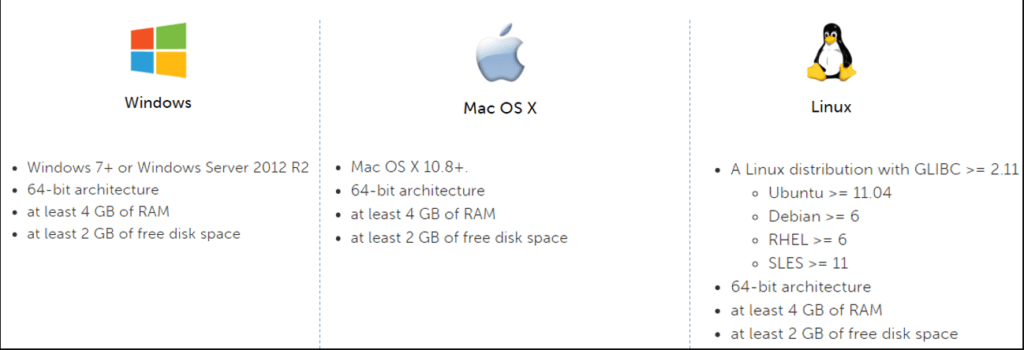
4. GraphLab only works on python 2. If you have Anaconda installed you can simple create a python 2 environment with the following commands.
![]()
Now activate the new environment –
![]()
5. If you are not using Anaconda, you can install python 2 from here
6. Once you have python 2 installed. It’s time to install GraphLab. Head over here to get the installation file.
There are two ways to install GraphLab –
Installation Method A
Using the GUI based tool to install it.

Download the installation file from the website and run it.

Enter your registered email address and the product key you received via email. And boom you are done.
Installation Method B
The second method to install GraphLab is via the pip package manager. Type the following commands to install GraphLab using pip –
pip install --upgrade --no-cache-dir https://get.graphlab.com/GraphLab-Create/2.1/your registered email address here/your product key here/GraphLab-Create-License.tar.gz
Using GraphLab to Conduct Churn Rate Analysis
Now that Graphlab is installed, the first step involves invoking the GraphLab package along with some other essential packages.
import graphlab as gl
import datetime
from dateutil import parser as datetime_parser
For reading in the CSV files we shall be using the SFrames from the GraphLab package.
sl = gl.SFrame.read_csv('online_retail.csv')
Parsing completed. Parsed 100 lines in 1.39481 secs.
------------------------------------------------------
Inferred types from first 100 line(s) of file as
column_type_hints=[long,str,str,long,str,float,long,str]
If parsing fails due to incorrect types, you can correct
the inferred type list above and pass it to read_csv in
the column_type_hints argument
------------------------------------------------------

Finished parsing file C:\Users\Rohit\Documents\Python Scripts\online_retail.csv
Parsing completed. Parsed 541909 lines in 1.22513 secs.
The file is read and parsed. Let’s have a look at the first few rows of the data set.
sl.head
From the above snippet of data set it’s apparent that the data set is transactional in nature, hence converting the SFrame to a time series is the preferred format. Before proceeding further, let’s convert the invoice date which is in the string format to date time format.
sl['InvoiceDate'] = sl['InvoiceDate'].apply(datetime_parser.parse)
Let’s confirm if the date is parsed in the right format as required.
sl.head
The invoice date column has indeed been parsed to the right format. The next step involves creating the time series with the invoice date as the reference.
timeseries = gl.TimeSeries(sl, 'InvoiceDate')
timeseries.head
The invoice date column has successfully been converted into a time series data set. Since, we don’t necessarily have a train-test data set. Let’s split the existing data set into a train and validation set.
train, valid = gl.churn_predictor.random_split(timeseries, user_id='CustomerID', fraction=0.7, seed = 2018)
This should split the existing data into 70% training and 30% validation. Before training the model on the train data set. We need to sort out a few things –
- We need to define the number of days after which a customer is categorised as churned,in this case it is 30 days.
- Since we need to look at the effectiveness of the algorithm, we need to set a date limit until which the algorithm trains on.
These two actions are accomplished with below code.
churn_period = datetime.timedelta(days = 30)
churn_boundary_oct = datetime.datetime(year = 2011, month = 8, day = 1)
Phew, finally let’s train the model.
model = gl.churn_predictor.create(train, user_id='CustomerID',
                  	features = ['Quantity'],
                  	churn_period = churn_period,
                  	time_boundaries = [churn_boundary_oct])
Here we are using only ‘quantity’ column as a dependent variable. Along with the churn_period and time_boundaries.
PROGRESS: Grouping observation_data by user.
PROGRESS: Resampling grouped observation_data by time-period 1 day, 0:00:00.
PROGRESS: Generating features at time-boundaries.
PROGRESS: --------------------------------------------------
PROGRESS: Features for 2011-08-01 05:30:00
PROGRESS: Training a classifier model.


Boosted trees classifier:
--------------------------------------------------------
Number of examples          : 2209
Number of classes           : 2
Number of feature columns   : 15
Number of unpacked features : 150
+-----------+--------------+-------------------+-------------------+
| Iteration | Elapsed Time | Training-accuracy | Training-log_loss |
+-----------+--------------+-------------------+-------------------+
| 1         | 0.015494     | 0.843821          | 0.568237          |
| 2         | 0.050637     | 0.856043          | 0.496491          |
| 3         | 0.062637     | 0.867361          | 0.445855          |
| 4         | 0.074637     | 0.871435          | 0.410984          |
| 5         | 0.086639     | 0.876415          | 0.386890          |
PROGRESS: --------------------------------------------------
PROGRESS: Model training complete: Next steps
PROGRESS: --------------------------------------------------
PROGRESS: (1) Evaluate the model at various timestamps in the past:
PROGRESS:       metrics = model.evaluate(data, time_in_past)
PROGRESS: (2) Make a churn forecast for a timestamp in the future:
PROGRESS:       predictions = model.predict(data, time_in_future)


| 6         | 0.094639     | 0.878225          | 0.369549          |
+-----------+--------------+-------------------+-------------------+
Hooray, the model has finished training. The next step involves evaluating the trained model. Since we have already split the data into train and validate, we need to evaluate the model on the validation set and not the training set. The model has been trained until the 1st of August 2011. And the churn time has been set to 30 days. We set the evaluation date to 1st September 2011.
evaluation_time = datetime.datetime(2011, 9, 1)
metrics = model.evaluate(valid, time_boundary = evaluation_time)
PROGRESS: Making a churn forecast for the time window:
PROGRESS: --------------------------------------------------
PROGRESS:  Start : 2011-09-01 00:00:00
PROGRESS:  End   : 2011-10-01 00:00:00
PROGRESS: --------------------------------------------------
PROGRESS: Grouping dataset by user.
PROGRESS: Resampling grouped observation_data by time-period 1 day, 0:00:00.
PROGRESS: Generating features for boundary 2011-09-01 00:00:00.
PROGRESS: Not enough data to make predictions for 321 user(s).
Metrics
{'auc': 0.7041731741781945, 'evaluation_data': Columns:
 	CustomerID	int
 	probability	float
 	label	int

 Rows: 1035

 Data:
 +------------+----------------+-------+
 | CustomerID |  probability   | label |
 +------------+----------------+-------+
 |   12365    | 0.899722337723 |   1   |
 |   12370    | 0.899722337723 |   1   |
 |   12372    | 0.877351164818 |   0   |
 |   12377    | 0.877230584621 |   1   |
 |   12384    | 0.879127502441 |   0   |
 |   12401    | 0.877230584621 |   1   |
 |   12402    | 0.877230584621 |   1   |
 |   12405    | 0.182979628444 |   1   |
 |   12414    | 0.90181106329  |   1   |
 |   12426    | 0.877351164818 |   1   |
 +------------+----------------+-------+
 [1035 rows x 3 columns]
 Note: Only the head of the SFrame is printed.
 You can use print_rows(num_rows=m, num_columns=n) to print more rows and columns., 'precision': 0.7741573033707865, 'precision_recall_curve': Columns:
 	cutoffs	float
 	precision	float
 	recall	float

 Rows: 5

 Data:
 +---------+----------------+----------------+
 | cutoffs |   precision    |     recall     |
 +---------+----------------+----------------+
 |   0.1   | 0.732546705998 | 0.997322623829 |
 |   0.25  | 0.753877973113 | 0.975903614458 |
 |   0.5   | 0.774157303371 | 0.922356091031 |
 |   0.75  | 0.801939058172 | 0.775100401606 |
 |   0.9   | 0.874345549738 | 0.223560910308 |
 +---------+----------------+----------------+
 [5 rows x 3 columns], 'recall': 0.9223560910307899, 'roc_curve': Columns:
 	threshold	float
 	fpr	float
 	tpr	float
 	p	int
 	n	int

 Rows: 100001

 Data:
 +-----------+-----+-----+-----+-----+
 | threshold | fpr | tpr |  p  |  n  |
 +-----------+-----+-----+-----+-----+
 |    0.0    | 1.0 | 1.0 | 747 | 288 |
 |   1e-05   | 1.0 | 1.0 | 747 | 288 |
 |   2e-05   | 1.0 | 1.0 | 747 | 288 |
 |   3e-05   | 1.0 | 1.0 | 747 | 288 |
 |   4e-05   | 1.0 | 1.0 | 747 | 288 |
 |   5e-05   | 1.0 | 1.0 | 747 | 288 |
 |   6e-05   | 1.0 | 1.0 | 747 | 288 |
 |   7e-05   | 1.0 | 1.0 | 747 | 288 |
 |   8e-05   | 1.0 | 1.0 | 747 | 288 |
 |   9e-05   | 1.0 | 1.0 | 747 | 288 |
 +-----------+-----+-----+-----+-----+
 [100001 rows x 5 columns]
 Note: Only the head of the SFrame is printed.
 You can use print_rows(num_rows=m, num_columns=n) to print more rows and columns.}
The Evaluation metrics such as AUC, precision and recall score are displayed in the report. However all the metrics can be obtained in a GUI.
time_boundary = datetime.datetime(2011, 9, 1)
view = model.views.evaluate(valid, time_boundary)
view.show()
PROGRESS: Making a churn forecast for the time window:
PROGRESS: --------------------------------------------------
PROGRESS:  Start : 2011-09-01 00:00:00
PROGRESS:  End   : 2011-10-01 00:00:00
PROGRESS: --------------------------------------------------
PROGRESS: Grouping dataset by user.
PROGRESS: Resampling grouped observation_data by time-period 1 day, 0:00:00.
PROGRESS: Generating features for boundary 2011-09-01 00:00:00.
PROGRESS: Not enough data to make predictions for 321 user(s).
PROGRESS: Making a churn forecast for the time window:
PROGRESS: --------------------------------------------------
PROGRESS:  Start : 2011-09-01 00:00:00
PROGRESS:  End   : 2011-10-01 00:00:00
PROGRESS: --------------------------------------------------
PROGRESS: Grouping dataset by user.
PROGRESS: Resampling grouped observation_data by time-period 1 day, 0:00:00.
PROGRESS: Generating features for boundary 2011-09-01 00:00:00.
PROGRESS: Not enough data to make predictions for 321 user(s)
We can pull out a report on the trained model using.
report = model.get_churn_report(valid, time_boundary = evaluation_time)
print report
+------------+-----------+----------------------+-------------------------------+
| segment_id | num_users | num_users_percentage |          explanation          |
+------------+-----------+----------------------+-------------------------------+
|     0      |    435    |    42.0289855072     | [No events in the last 21 ... |
|     1      |    101    |    9.75845410628     | [Less than 2.50 days with ... |
|     2      |     80    |    7.72946859903     | [No "Quantity" events in t... |
|     3      |     51    |    4.92753623188     | [No events in the last 21 ... |
|     4      |     51    |    4.92753623188     | [Less than 28.50 days sinc... |
|     5      |     44    |    4.25120772947     | [Greater than (or equal to... |
|     6      |     36    |    3.47826086957     | [No events in the last 21 ... |
|     7      |     32    |    3.09178743961     | [Less than 2.50 days with ... |
|     8      |     24    |    2.31884057971     | [Sum of "Quantity" in the ... |
|     9      |     22    |    2.12560386473     | [Greater than (or equal to... |
+------------+-----------+----------------------+-------------------------------+
+-----------------+------------------+-------------------------------+
| avg_probability | stdv_probability |             users             |
+-----------------+------------------+-------------------------------+
|  0.897792713258 | 0.0240167598568  | [12365, 12370, 12372, 1237... |
|  0.69319883166  |  0.100162972963  | [12530, 12576, 12648, 1269... |
|  0.757627598941 | 0.0904122072578  | [12432, 12463, 12465, 1248... |
|  0.859993882623 |  0.070536854901  | [12384, 12494, 12929, 1297... |
|  0.792790167472 | 0.0859747592324  | [12513, 12556, 12635, 1263... |
|  0.25629338131  |  0.135935808077  | [12471, 12474, 12540, 1262... |
|  0.866931213273 |  0.034443289173  | [12548, 12818, 16832, 1688... |
|  0.632504582405 |  0.121735932946  | [12449, 12500, 12624, 1263... |
|  0.824982141455 | 0.0968270683383  | [12676, 12942, 12993, 1682... |
| 0.0796884274618 | 0.0453845944586  | [12682, 12748, 12901, 1667... |
+-----------------+------------------+-------------------------------+
[46 rows x 7 columns]
Note: Only the head of the SFrame is printed.
You can use print_rows(num_rows=m, num_columns=n) to print more rows and columns.
The training data used for the model along with the features created for the data can be viewed by.
Model.processed_training_data.head

print model.get_feature_importance()
+-------------------------+-------------------------------+-------+
|           name          |             index             | count |
+-------------------------+-------------------------------+-------+
|  Quantity||features||7  |       user_timesinceseen      |   62  |
|  Quantity||features||90 |            sum||sum           |   24  |
|  __internal__count||90  |           count||sum          |   20  |
|  Quantity||features||60 |            sum||sum           |   15  |
|  Quantity||features||90 |           sum||ratio          |   14  |
|  Quantity||features||7  |            sum||sum           |   13  |
| UnitPrice||features||90 |            sum||sum           |   12  |
| UnitPrice||features||60 |            sum||sum           |   12  |
|  Quantity||features||90 |           sum||slope          |   11  |
|  Quantity||features||90 | sum||firstinteraction_time... |   11  |
+-------------------------+-------------------------------+-------+
+-------------------------------+
|          description          |
+-------------------------------+
|  Days since most recent event |
| Sum of "Quantity" in the l... |
|   Events in the last 90 days  |
| Sum of "Quantity" in the l... |
| Average of "Quantity" in t... |
| Sum of "Quantity" in the l... |
| Sum of "UnitPrice" in the ... |
| Sum of "UnitPrice" in the ... |
| 90 day trend in the number... |
| Days since the first event... |
+-------------------------------+
[150 rows x 4 columns]
Note: Only the head of the SFrame is printed.
You can use print_rows(num_rows=m, num_columns=n) to print more rows and columns.
The last and final part in the exercise is to predict which customers might churn. This is done on the validation data set.
predictions = model.predict(valid, time_boundary= evaluation_time)
predictions.head
The values given in the 2nd column are the probability that a user will have no activity in the churn period that we defined earlier (30 days), hence the probability for the customer to churn. You can obtain the prediction for the first 500 customers by using
predictions.print_rows(num_rows = 10000)
You can adjust the number of predictions to be displayed using
num_rows
Conclusion
Now that we have discussed a way to calculate churn with unlabelled data, it’s your turn to use the methods discussed to experiment with the GraphLab package.
And if you enjoyed this demonstration, consider enrolling in our course on Python for Data Science over on LinkedIn Learning.


